Examples & Results

Runnable examples for the Python API, then the published benchmark results and how to reproduce them.

Important

October 7 update: the complete corrected campaign with all baselines ran on the shipped code in a quiet window — see Current code — full campaign below. October 5: the audit-fixed kernel’s same-machine A/B completed with identical matched quality counts; 19/20 cells were consistently faster and one approximately unchanged. This is not a rerun against the paper’s hardware or competitor baselines. The later dependency pin update (GRiD/GLASS) was confirmed separately on October 6: identical matched quality counts and paired latency ratios within 0.9946–1.0046 (unchanged); see the repository’s docs/development/evidence/audit_timing_2026-10-05/ and evidence/postpin_timing_2026-10-06/ for exact provenance and ratios. The October 2 A/B driver forced fp32 even for S=1; it did not exercise default S=1 fp64. October 3 conservative-model ladder dumps omitted empty outputs (b10: 2775, b15: 2771 of 2776 queries); those groups were recollected on October 7 with identical cage rates (fairness_hardsets_2026-10-03/recollection_2026-10-07). Default-model groups were complete. New dumps retain empty queries and target/frame metadata for independent FK. Archived tables/plots below are historical evidence, not a new guarantee of final-code performance. Visual-mesh judges exclude base/self collision and shrink obstacles by the stated tolerance; they are not physical ground truth.

Examples

Self-contained, runnable programs live in the repository’s examples/ directory. Each is included in full below (so the docs never drift from the code). Run any with the project’s virtual environment active, e.g. python examples/01_open_world_solve.py.

Example	Shows	Needs
01_open_world_solve	Batch-solve one 6-DOF target; inspect the best returned solutions	built hjcdik
02_collision_free_solve	Collision-free solve against a MotionBenchMaker scene (obstacles on GPU)	grasptarget build
03_batch_sweep	How the best-solution accuracy improves with batch size	built hjcdik

01 — Open-world solve

"""01 — Open-world IK: batch-solve a single 6-DOF target.

Generate many candidate solutions in parallel for one end-effector pose, then inspect the best ones.
Run: ``python examples/01_open_world_solve.py``
"""
from hjcdik import generate_solutions, sample_targets, num_joints

print(f"robot DOF: {num_joints()}")

# A reachable target pose: [x, y, z, qw, qx, qy, qz] (position + unit quaternion).
target = sample_targets(num_targets=1, seed=0)[0]
print("target:", target)

# Explore 2000 candidates in parallel; request up to 4 distinct solutions.
out = generate_solutions(target, batch_size=2000, num_solutions=4)

print(f"returned {out['count']} solutions")
print("joint configs shape:", out["joint_config"].shape)   # (count, DOF)
if out["count"]:
    # Keep the two errors paired: their separate minima can belong to different candidates.
    for i, (pos, ori) in enumerate(zip(out["pos_errors"], out["ori_errors"])):
        print(f"candidate {i}: position (mm)={pos:.3e}, orientation (rad)={ori:.3e}")
    acceptable = (out["pos_errors"] < 1.0) & (out["ori_errors"] < 0.001)
    print("candidates within 1 mm and 0.001 rad:", out["joint_config"][acceptable])
else:
    print("No candidate was returned.")
# A returned candidate is approximate: check BOTH errors against your tolerances.

02 — Collision-free solve

The scene and goal come from tests/mb_problems.json; the GPU filters candidates against the obstacles in the chosen problem set (the Results section below covers the benchmark harness and reproduction).

"""02 — Collision-free IK against a MotionBenchMaker scene.

Solve IK while the GPU filters candidates against the obstacles in a problem set. The scene + goal come
from ``tests/mb_problems.json`` (the same sets the benchmark uses). Requires HJCD-IK built with the
``panda_grasptarget_hand`` frame (the committed default). Dataset goals describe panda_hand;
the fixed tool offset is applied explicitly below to preserve the requested hand pose.

Run: ``python examples/02_collision_free_solve.py``
"""
import json
import sys
from pathlib import Path

from hjcdik import generate_solutions, build_info

sys.path.insert(0, str(Path(__file__).resolve().parents[1] / "benchmark"))
from query_results import panda_hand_target, best_candidate

PROBLEMS = Path(__file__).resolve().parents[1] / "tests" / "mb_problems.json"
PROBLEM_SET = "box_panda"
PROBLEM_IDX = 0

problems_text = PROBLEMS.read_text()
problem = json.loads(problems_text)["problems"][PROBLEM_SET][PROBLEM_IDX]

# Goal pose for this problem: [x, y, z, qw, qx, qy, qz].
gp = problem["goal_pose"]
target = [*gp["position_xyz"], *gp["quaternion_wxyz"]]
target = panda_hand_target(target, build_info()["ee_target"])

out = generate_solutions(
    target,
    batch_size=2000,
    num_solutions=4,
    collision_free=True,
    collision_mode="hard",
    problems_json_text=problems_text,   # the GPU reads obstacles from this set...
    problem_set_name=PROBLEM_SET,
    problem_idx=PROBLEM_IDX,             # ...for this specific scene
)

print(f"set={PROBLEM_SET} idx={PROBLEM_IDX}: {out['count']} collision-free solutions")
if out["count"]:
    best = best_candidate(out)
    print("selected candidate position error (mm):  ", float(out["pos_errors"][best]))
    print("selected candidate orientation error (rad):", float(out["ori_errors"][best]))
    print("within 5 mm and 0.05 rad:", bool(out["pos_errors"][best] < 5 and out["ori_errors"][best] < .05))
else:
    print("No collision-free candidate was found in this batch.")

03 — Batch-size sweep

"""03 — Batch-size sweep: accuracy vs. batch size.

Larger batches explore more candidates for ONE target. Coarse search uses one block per
candidate; refinement uses one warp per candidate. This reports accuracy, not performance:
accuracy need not improve monotonically, and runtime depends on hardware and settings.

Run: ``python examples/03_batch_sweep.py``
"""
from hjcdik import generate_solutions, sample_targets

target = sample_targets(num_targets=1, seed=0)[0]

print(f"{'batch':>8}  {'best pos err (mm)':>18}  {'best ori err (rad)':>20}")
for batch in (1, 10, 100, 1000, 2000):
    out = generate_solutions(target, batch_size=batch, num_solutions=1)
    if out["count"]:
        print(f"{batch:>8}  {float(out['pos_errors'].min()):>18.3e}  {float(out['ori_errors'].min()):>20.3e}")
    else:
        print(f"{batch:>8}  no candidate returned")

Results

In the published experiments below, HJCD-IK stayed on or near the accuracy–latency Pareto frontier across the evaluated batch sizes and degree-of-freedom counts, with order-of-magnitude gains in some comparisons and the lowest measured MMD. These are historical paper results, not new measurements of the current release.

Note

All numbers below are from the camera-ready paper (arXiv:2510.07514, IROS 2026) — the single source of truth. They were collected on an NVIDIA RTX 4060 (Intel i7-14700HX, WSL Ubuntu 24.04, CUDA 12.5) over 100 Halton open-world poses and the box_panda MotionBenchMaker scene. Benchmarks you run locally (see Reproducing these results, below) are for your own validation and will differ with hardware. Position error is in mm, orientation error in rad, time in ms; bold marks the best (HJCD-IK) value.

Open-world IK — Panda (Table I)

Batch	HJCD-IK Time	HJCD-IK Pos	HJCD-IK Ori	PyRoki Time	PyRoki Pos	PyRoki Ori	cuRobo Time	cuRobo Pos	cuRobo Ori	IKFlow Time	IKFlow Pos	IKFlow Ori
1	4.04	7.04e-2	2.04e-3	14.86	1.39e-2	1.12e-5	5.33	2.56e1	1.11e-1	18.48	4.67e0	2.28e-2
10	3.82	1.21e-4	6.74e-7	14.62	1.39e-2	1.12e-5	5.55	2.49e-3	3.95e-6	18.95	1.38e0	6.21e-3
100	4.07	2.25e-5	8.95e-8	14.20	1.39e-2	1.12e-5	6.01	9.16e-4	2.83e-6	22.29	5.94e-1	2.76e-3
1000	4.22	1.60e-5	9.15e-8	13.96	1.39e-2	1.12e-5	19.80	3.67e-4	1.68e-6	49.78	2.06e0	5.43e-3
2000	4.37	1.81e-5	5.15e-8	13.97	1.39e-2	1.12e-5	30.30	2.65e-4	1.33e-6	99.98	1.92e0	6.59e-3

Open-world IK — Fetch (Table I)

Batch	HJCD-IK Time	HJCD-IK Pos	HJCD-IK Ori	PyRoki Time	PyRoki Pos	PyRoki Ori	cuRobo Time	cuRobo Pos	cuRobo Ori	IKFlow Time	IKFlow Pos	IKFlow Ori
1	2.59	5.79e-1	1.20e-3	13.70	2.10e-5	3.12e-8	5.30	4.48e0	3.70e-3	17.40	1.92e1	6.67e-2
10	2.41	1.40e-6	9.56e-9	13.48	2.10e-5	3.12e-8	5.52	6.74e-4	1.08e-6	16.36	9.60e0	3.66e-2
100	2.52	1.67e-6	8.97e-9	13.16	2.10e-5	3.12e-8	7.57	1.61e-4	8.87e-7	19.75	1.65e1	7.24e-2
1000	2.59	1.67e-6	6.10e-9	12.92	2.10e-5	3.12e-8	11.32	5.17e-5	6.43e-7	48.68	2.05e1	6.03e-2
2000	2.73	1.66e-6	9.70e-9	13.37	2.10e-5	3.12e-8	14.62	3.96e-5	5.94e-7	87.89	1.52e1	4.87e-2

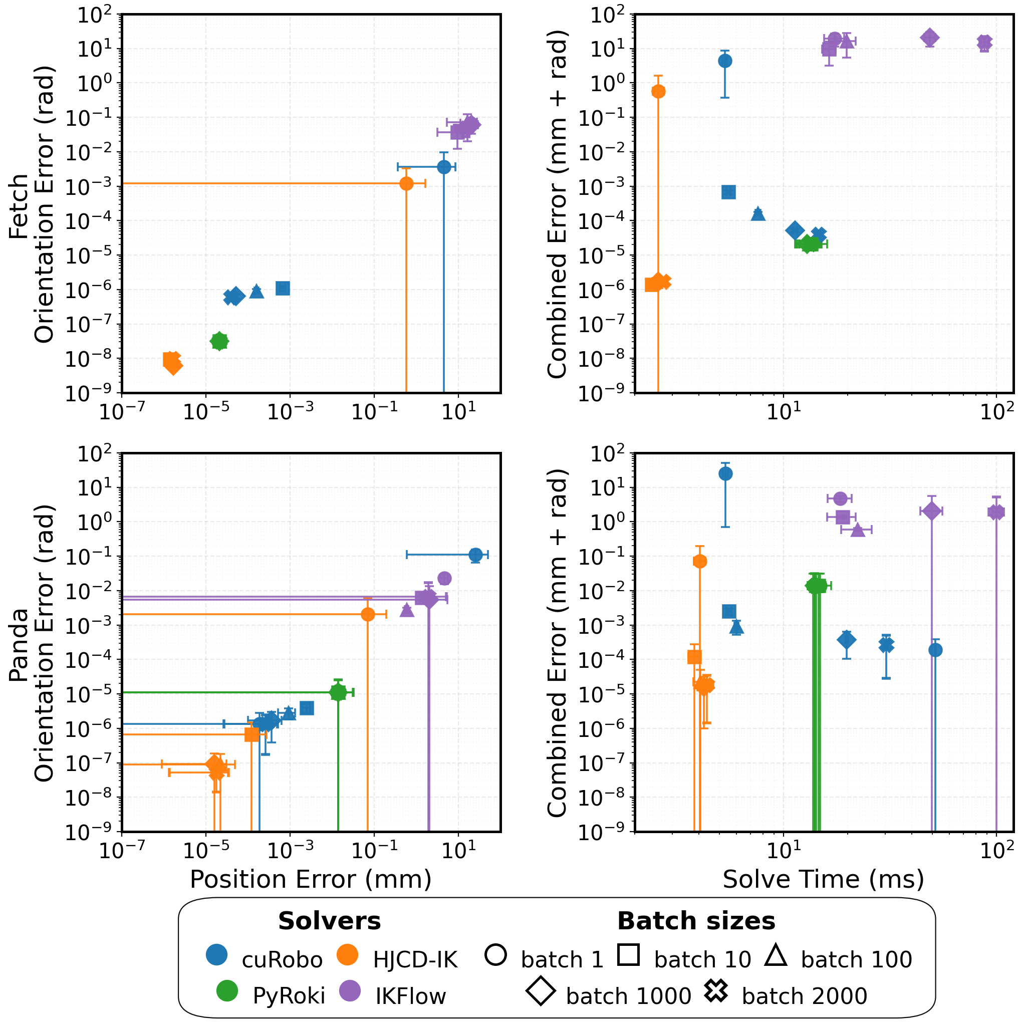
Fig. 2 Open-world accuracy–latency frontier (Table I) — HJCD-IK (orange), cuRobo (blue), PyRoki (green).

Collision-free IK — Panda, box_panda (Table II)

Batch	HJCD-IK Time	HJCD-IK Pos	HJCD-IK Ori	HJCD-IK Succ	PyRoki Time	PyRoki Pos	PyRoki Ori	PyRoki Succ	cuRobo Time	cuRobo Pos	cuRobo Ori	cuRobo Succ
1	5.44	8.17	1.96e-2	89.0	34.04	5.18e2	3.96e-1	6.0	23.76	7.85	2.61e-3	97.0
10	4.19	7.11e-4	5.34e-7	98.0	46.29	9.90e-5	1.69e-7	89.0	29.31	2.43e-3	4.00e-6	100.0
100	4.42	8.83e-5	3.56e-8	100.0	48.98	9.80e-5	1.41e-7	93.0	30.76	6.99e-4	2.00e-6	100.0
1000	5.04	2.03e-5	9.06e-9	100.0	46.98	8.70e-5	1.36e-7	92.0	28.50	2.93e-4	2.00e-6	100.0
2000	5.35	1.71e-5	7.16e-9	100.0	35.74	8.80e-5	1.49e-7	90.0	61.96	2.47e-4	2.00e-6	100.0

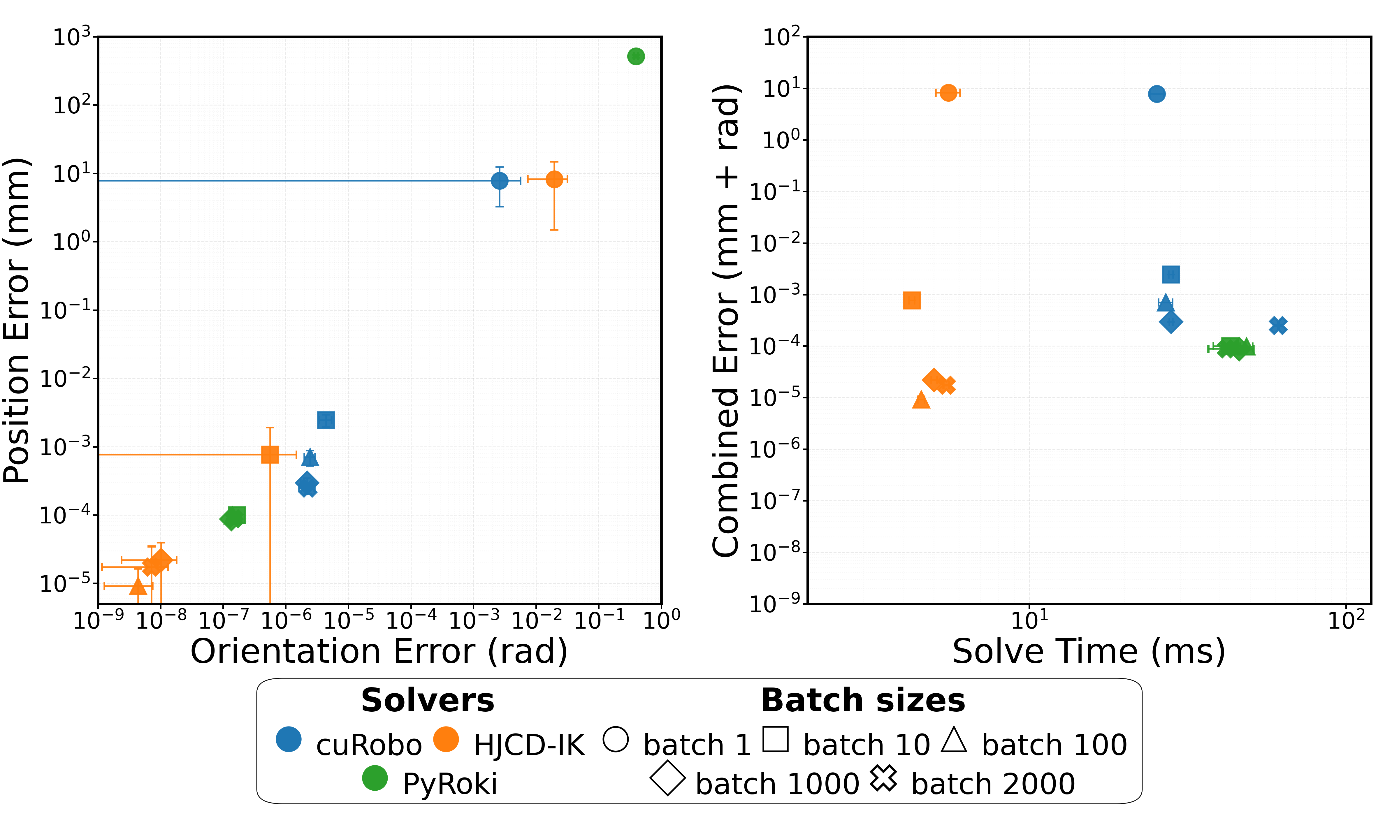
Fig. 3 Collision-free frontier on the box_panda scene (Fig. 4, Table II).

Note

Collision-free validation (methodology). The local benchmark tools validate returned configurations post-hoc against the legacy paper 59-sphere Panda model (benchmark/panda_collision.py, sourced from the frozen benchmark/reference/panda_collision_model.cuh). This is an environment-only check. It is not identical to HJCD-IK’s compiled URDF-driven model: the paper reference uses +/-65 mm finger-joint origins, whereas the compiled kinematic URDF uses +/-40 mm. Four finger-sphere centers consequently differ by 25 mm. Self-collision exclusions also follow the generated topology rather than this environment-only oracle. Shared geometry makes the environment predicate comparable, but does not make all reported percentages equivalent: HJCD’s collision column is per returned solution; a baseline success_both combines pose success and collision freedom. Account for missing outputs and align denominators/accuracy thresholds before making a cross-solver success-rate table. The check is pure NumPy (no cuRobo dependency). Run benchmark/baseline_bench.py --mode {pyroki,curobo} --collision_free (per-run CSV/YAML land under the gitignored benchmark/results/; the time/accuracy numbers above are the camera-ready values).

HJCD’s harness preserves this comparison with --collision-validation-model paper (default). Select --collision-validation-model hjcd for an independent CPU check of its current URDF-bound sphere geometry instead; this does not change the solver model. Do not mix those rates in one cross-solver table. Collision CSV/YAML outputs also write <output>.metadata.json with validation model, source hashes, finger origins, and the compiled header identity. Historical result files without that sidecar retain their original paper-model interpretation.

DoF scalability — Panda variants, B = 1000 (Table III)

DoF	HJCD-IK Time	HJCD-IK Pos	HJCD-IK Ori	PyRoki Time	PyRoki Pos	PyRoki Ori	cuRobo Time	cuRobo Pos	cuRobo Ori
7	4.25	1.71e-5	4.11e-8	15.09	2.63e-2	3.70e-5	9.11	3.38e-4	1.59e-6
12	4.55	1.94e-5	6.91e-8	16.29	1.99e-2	1.86e-5	12.66	7.78e-1	2.57e-2
18	4.62	3.76e-5	6.95e-8	20.82	2.15e-2	2.14e-5	16.26	8.41e-1	3.03e-2
24	4.66	3.84e-5	7.32e-8	24.34	1.84e-2	1.99e-5	19.55	7.50e-1	3.58e-2

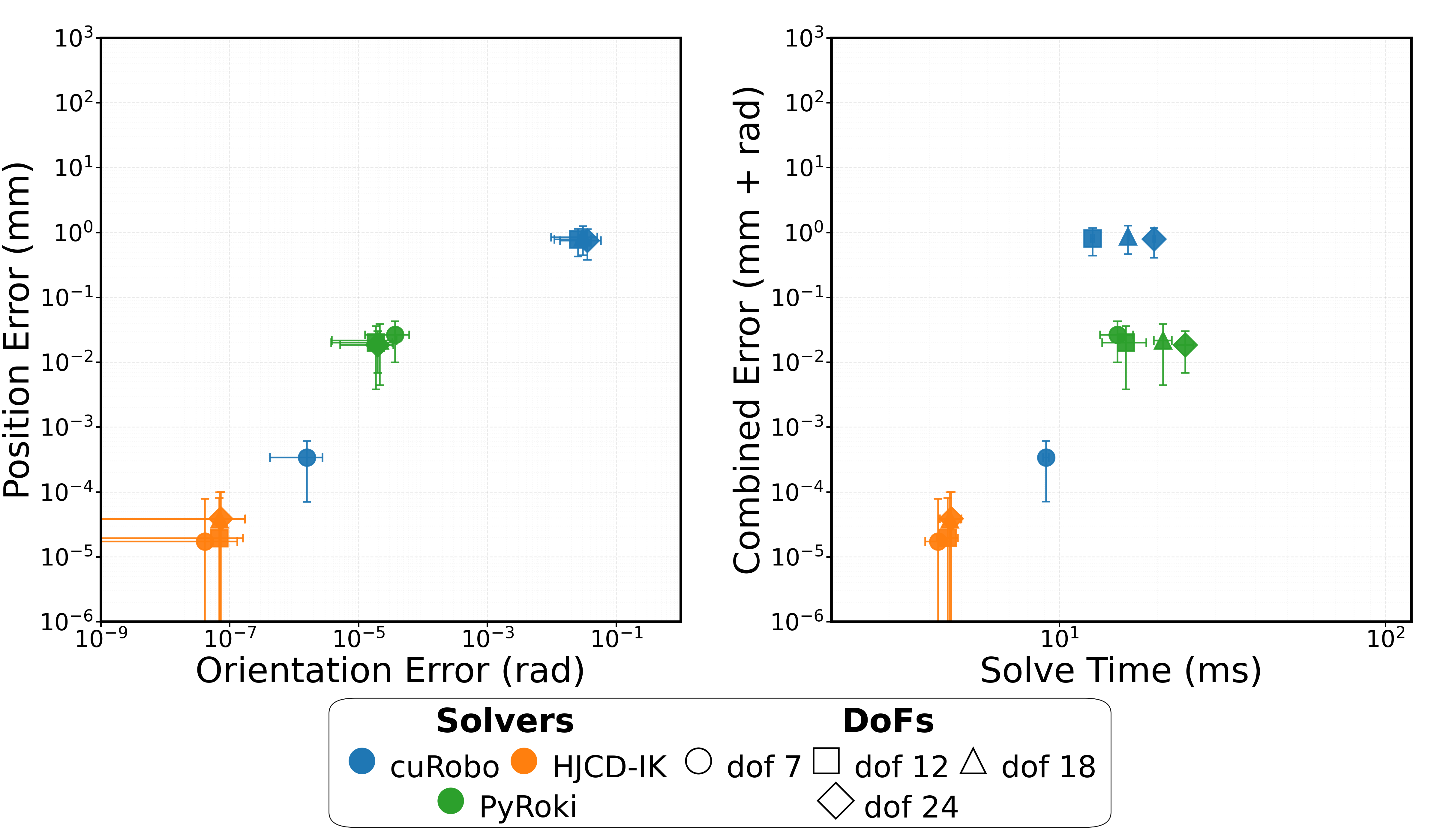
Fig. 4 DoF scaling, 7–24 DoF (Fig. 5, Table III) — HJCD-IK keeps the lowest error and latency at every DoF.

Solution diversity — MMD vs. TRAC-IK (Table IV)

Maximum Mean Discrepancy between each solver’s 50 best configurations (of a batch of 2000) and 50 ground-truth samples, over 100 target poses — lower is a closer match to the full IK manifold.

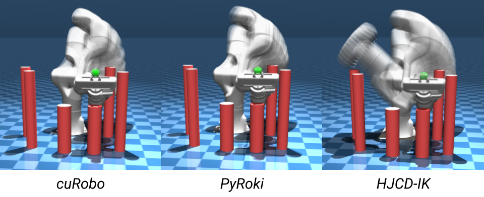
Fig. 5 Distribution of collision-free IK solutions for a representative target — cuRobo (left), PyRoki (center), HJCD-IK (right). HJCD-IK returns a broader, more diverse spread of locally-optimal solutions.

Current code — full campaign, RTX 5090, 2026-10-07

Note

This is the complete, corrected campaign on the shipped code (main at f4dc1b5; solver identical to the pushed dd4c350) with every baseline installed and collision-constrained, run in a user-announced quiet window (exit 0, 1604 s, no stage skipped, no foreign GPU process; see docs/development/evidence/paper_rerun_2026-10-07/). Different GPU, different cuRobo generation and a corrected protocol from the camera-ready tables above — never mix the two. Time is the mean per-call wall time; position error is the mean over 100 queries.

Open-world, Panda (100 Halton targets, panda_hand): time in ms / position error in mm.

Batch	HJCD-IK	cuRobo v2	PyRoki	IKFlow
1	3.30 / 2.80 (95/100 within 5 mm)	8.52 / 1.8e-2	3.30 / 371	2.60 / 16.0
10	2.04 / 5.8e-5	5.90 / 1.7e-2	5.62 / 5.2	2.48 / 3.3
100	1.65 / 1.8e-5	5.93 / 1.8e-2	6.02 / 0.39	2.76 / 1.7
1000	1.62 / 4.2e-5	6.14 / 2.1e-2	7.04 / 1.1e-4	5.10 / 0.77
2000	1.65 / 2.5e-5	6.35 / 2.1e-2	7.19 / 1.2e-4	6.15 / 0.70

Fetch open-world: HJCD-IK 0.81–1.10 ms (100 % within 5 mm at every batch), cuRobo v2 1.81–2.10 ms, PyRoki 2.8–6.0 ms, IKFlow 2.5–6.2 ms (30–160 mm error). DoF scaling at B = 1000 (7 / 12 / 18 / 24 DoF): HJCD-IK 1.76 / 1.87 / 2.31 / 2.85 ms, cuRobo v2 2.38 (median; its mean of 8.74 contains one 591 ms kernel JIT on the first problem) / 2.19 / 2.45 / 2.67 ms, PyRoki 6.8 / 8.2 / 10.7 / 12.7 ms. MMD (lower is better): HJCD-IK 0.098, PyRoki 0.124, cuRobo v2 0.143, IKFlow 0.211.

Collision-free, every solver collision-constrained, B = 2000, 100 problems per set: mean ms / success (pose < 5 mm and < 0.05 rad and collision-free under the visual-mesh judge at 1 mm, on the stored configurations). PyRoki here runs its world/self-collision costs on the foam spheres (the October 3 PyRoki latencies were plain IK and are not comparable).

Set (dataset protocol unless noted)	HJCD-IK	cuRobo v2	PyRoki
box (paper protocol: TCP, cylinder-snapped)	1.82 / 100 %	2.45 / 100 %	29.1 / 100 %
box	2.10 / 100 %	2.44 / 100 %	30.3 / 100 %
bookshelf_small	2.10 / 100 %	2.49 / 98 %	29.1 / 100 %
bookshelf_tall	2.07 / 100 %	2.46 / 100 %	30.6 / 100 %
bookshelf_thin	1.82 / 100 %	2.45 / 100 %	32.9 / 100 %
cage	1.86 / 100 %	2.46 / 100 %	26.9 / 100 %
table_pick	2.64 / 100 %	2.43 / 99 %	32.5 / 100 %
table_under_pick	2.34 / 100 %	2.44 / 98 %	30.9 / 100 %
kitchen	1.83 / 99 %	2.44 / 99 %	37.7 / 99 %
table_bars	3.22 / 100 %	2.47 / 100 %	27.1 / 100 %

At B = 100, HJCD-IK is 98–100 % on every set (cuRobo 97–100 %, PyRoki 95–100 %) at 1.7–3.0 ms. With one candidate (B = 1) HJCD-IK’s collision-free success is 5–95 % depending on the set: the single-candidate regime is not where a batched solver is meant to run. The harder clearance-ladder results, the judges and the sphere-model analysis are in the fairness section further down; they were not re-timed.

Historical rerun — RTX 5090, 2026-10-03

Note

This section records the October 3 snapshot, starting at 2fc1316 with the follow-up fixes identified in its evidence directories. It is not a measurement of today’s HEAD. It used the then-installed competitor versions (cuRobo v2 main, PyRoki main, IKFlow 0.0.8) on an RTX 5090 with CUDA 13. It does not replace the camera-ready tables above and must not be mixed with them: different GPU, different cuRobo generation, and — for the collision scenes — a corrected evaluation protocol. Full raw data, logs and caveats: docs/development/evidence/paper_rerun_2026-10-03/ (latency campaign) and docs/development/evidence/fairness_hardsets_2026-10-03/ (collision judges, clearance ladder, new sets).

What changed in the protocol. The MotionBenchMaker goals are panda_hand poses (the dataset’s own IK solutions put panda_hand on them; the TCP is 105 mm further along the approach axis). The paper’s Table II snapped the target onto the grasped cylinder and solved for the TCP, which is physically consistent for cylinder-grasp scenes such as box_panda but is undefined for scenes without a cylinder near the goal. The rerun therefore reports two protocols: the paper protocol on box_panda for continuity, and the dataset protocol (panda_hand frame, goal_pose exactly as posed, every solver at the same frame) on all eight MotionBenchMaker sets (plus kitchen and table_bars below). Collision claims are scored on the stored configurations by independent judges — the true-geometry mesh as the headline, sphere models and the convex-hull meshes alongside (see All MotionBenchMaker sets below); the collision_free column of the raw CSVs is the shared hjcd sphere oracle.

Open-world, Panda (100 Halton targets, panda_hand): time in ms, position error in mm.

Batch	HJCD-IK Time	HJCD-IK Pos	cuRobo v2 Time	cuRobo v2 Pos	PyRoki Time	PyRoki Pos	IKFlow Time	IKFlow Pos
1	3.34	2.80 (5/100 miss)	8.55	1.82e-2	3.26	371	2.69	13.3
10	2.08	5.77e-5	5.97	1.73e-2	5.40	5.22	2.57	3.70
100	1.67	2.28e-5	6.02	1.78e-2	5.63	0.390	2.86	1.49
1000	1.72	4.80e-5	6.25	2.09e-2	6.86	1.08e-4	5.14	0.732
2000	1.75	4.99e-5	6.43	2.09e-2	6.87	1.13e-4	6.19	0.653

Fetch open-world: HJCD-IK 0.82–1.11 ms, cuRobo v2 1.85–2.22 ms, PyRoki 3.1–6.1 ms, IKFlow 2.6–6.2 ms (31–137 mm error). DoF scaling at B = 1000 (7 / 12 / 18 / 24 DoF): HJCD-IK 1.80 / 1.89 / 2.39 / 2.99 ms, cuRobo v2 2.02 / 2.17 / 2.49 / 2.68 ms, PyRoki 7.0 / 8.8 / 10.4 / 13.0 ms. MMD (lower is better): HJCD-IK 0.103, PyRoki 0.128, cuRobo v2 0.144, IKFlow 0.222.

Collision-free, box_panda, both protocols (time ms / position error mm at B = 2000, 100 problems):

Protocol	HJCD-IK	cuRobo v2	PyRoki
Paper (TCP, cylinder-snapped target)	2.26 / 9.9e-6	2.47 / 1.6e-5	7.22 / 1.2e-4
Dataset (panda_hand, goal as posed)	2.55 / 4.7e-6	2.51 / 2.1e-3	7.73 / 1.1e-4

All MotionBenchMaker sets, every solver collision-constrained (dataset protocol, B = 2000, 100 problems each). Success means the returned configuration both reaches the pose (< 5 mm, < 0.05 rad) and is collision-free. Three judges score the stored configurations (benchmark/score_collision_oracles.py): the headline is the visual-mesh approximation (the panda_description visual meshes under FCL, obstacles shrunk by 1 mm so touching is permitted); beside it, in small type, the solver’s own sphere model (foam’s 58 spheres for HJCD-IK and PyRoki, cuRobo’s 61 for cuRobo) and the convex hull judge (the stock panda_description collision meshes, which are convex hulls — MoveIt’s and MotionBenchMaker’s own geometry; link 5’s hull is 50 % larger than the link). PyRoki runs PyRoki’s world- and self-collision costs on the foam spheres (its URDF capsule model is 16–70 mm too coarse for these gaps); cuRobo runs its bundled sphere model. Two HJCD-IK columns: the kernel before and after the collision-aware refinement described below, and a third compiled on cuRobo’s sphere model instead of foam’s (benchmark/make_curobo_sphere_urdf.py) — the controlled experiment that separates the collision model from the search. kitchen and table_bars are MotionBenchMaker scenes exported from the public dataset (benchmark/mbm_export.py; mesh furniture decomposed exactly into boxes and cylinders), new here.

Set	HJCD-IK (before)		HJCD-IK		HJCD-IK / cuRobo spheres		cuRobo v2		PyRoki
	true mesh	own / hull	true mesh	own / hull	true mesh	own / hull	true mesh	own / hull	true mesh	own / hull
bookshelf_small	99	100 / 94	100	100 / 95	100	100 / 95	98	98 / 93	100	100 / 98
bookshelf_tall	100	100 / 98	100	100 / 98	100	100 / 98	100	100 / 98	100	100 / 100
bookshelf_thin	100	100 / 100	100	100 / 100	100	100 / 100	100	100 / 100	100	100 / 100
box	100	100 / 100	100	100 / 100	100	100 / 100	100	100 / 100	100	100 / 100
box_flipped	100	100 / 100	100	100 / 100	100	100 / 100	100	100 / 100	100	100 / 100
cage	96	97 / 78	100	100 / 87	100	100 / 86	100	100 / 77	100	100 / 80
table_pick	94	95 / 90	100	100 / 95	97	100 / 92	99	100 / 95	100	100 / 98
table_under_pick	95	95 / 95	100	100 / 99	97	100 / 94	98	100 / 95	100	100 / 100
kitchen	99	99 / 99	99	99 / 99	100	100 / 100	99	100 / 99	99	99 / 99
table_bars	100	100 / 72	100	100 / 69	98	100 / 66	100	100 / 33	100	100 / 71

Collision-aware refinement (kernel change, 2026-10-03). The cross-block early stop used to be raised by the first pose-accurate candidate, colliding or not, so in a cluttered scene the whole batch could stop on a candidate the hard filter then discarded. In hard/both collision modes the kernel now (i) raises the stop only for a collision-free accurate candidate, decided warp-locally from the joint transforms the solver already holds (grid_collision::warp::config_free: spheres placed from GRiD-generated tables in grid.cuh, no block barrier, no extra FK; the original HJCD sidecar has been removed); (ii) ranks the LM seeds with a penalty on colliding coarse candidates; (iii) gives an accurate-but-colliding LM candidate an informed repair round — a deterministic joint-space kick that grows per attempt, after which the LM re-projects it onto the pose and the verdict is re-run (HJCD_REPAIR_ATTEMPTS, default 4); and (iv) keeps the best collision-free configuration inside the success band (5 mm / 0.05 rad) as a fallback when the exactly converged free candidate was not found in this run. Open-world solves never enter this collision-policy path. The October 5 A/B gate above covers the subsequent audit-fixed kernel; the later dependency-pin confirmation remains separate. The archived October 3 effect on three dataset sets was cage 96 → 100 %, table_pick 94 → 100 %, table_under_pick 95 → 100 %; those are observed counts, not guaranteed success. The audit’s complete ten-set recollection at B=2000 solved 999/1000 queries (one kitchen miss). Nonempty output is not necessarily pose-accurate, and harder ladder scenes have misses. Two follow-ups closed on October 7 (shared GPU, correctness only): success is now monotone in the batch size on the hard sets (cage 99/100/100/100 %, table_pick 98/100/100/100 %, table_under_pick 99/99/100/100 % at B = 100/1000/2000/8000; docs/development/evidence/c1_batch_monotonic_2026-10-07/), and a nullspace repair step (contact normals from grid_collision::warp::collision_distance projected onto the end-effector Jacobian’s nullspace, then LM re-projection) was implemented and measured on the full ladder against the shipped kick: 2545 vs 2547 of 2776 queries — a wash — because in every cell the solver never returns an accurate configuration its own spheres reject, so there is nothing left for a repair step to act on; the remaining misses belong to the sphere model. It was not shipped (docs/development/evidence/repair_nullspace_2026-10-07/).

Clearance ladder. To see where the solvers separate, every cuboid of the three tightest sets is grown by D on each face (benchmark/make_clearance_ladder.py), keeping only problems for which at least one of the dataset’s own goal_ik solutions is still free under the hull judge (so every kept problem is known-feasible). Success under the visual-mesh judge vs D, B = 100 (solid) and 2000 (dashed):

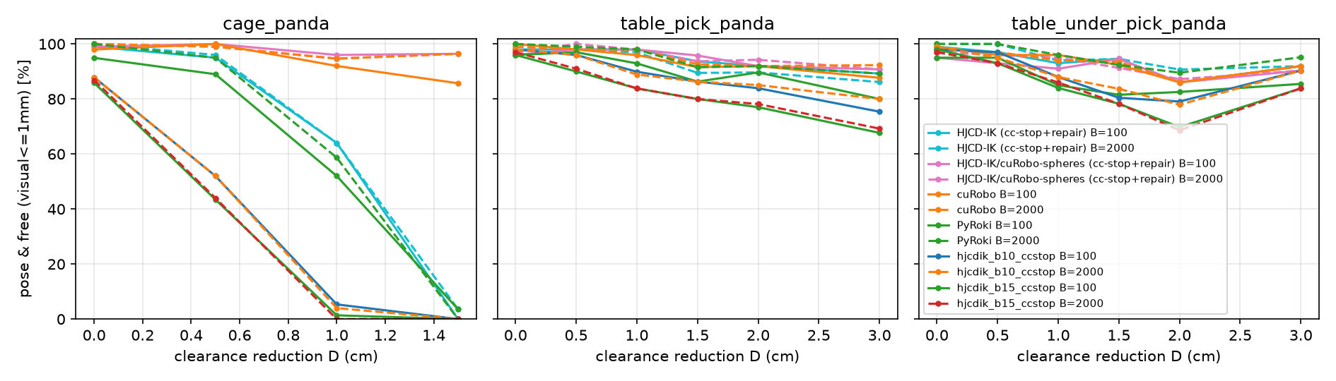
Fig. 6 Success (pose reached and collision-free under the visual meshes, 1 mm) against the clearance reduction D. Kept problems per level: cage 99 / 100 / 75 / 28; table_pick 100 / 100 / 99 / 95 / 87 / 65; table_under_pick 100 / 100 / 100 / 92 / 86 / 62 (D = 0 / 0.5 / 1 / 1.5 / 2 / 3 cm). “b10”/”b15” are the bounded-bulge models of the fidelity table below.

With the refinement, HJCD-IK on its own foam spheres is within 0–4 points of cuRobo at every table level (B = 2000: table_pick 100/98/97/89/90/86 vs 99/98/98/93/92/92; table_under_pick 100/100/94/95/91/92 vs 98/97/94/93/86/92) and above it on several. In the cage it still falls to 64 % at D = 1 cm and 4 % at 1.5 cm while cuRobo holds 95–96 %. Model substitution strongly implicates geometry in this gap: HJCD-IK compiled on cuRobo’s spheres scores 95 % and 96 % there — identical to cuRobo. The table below says why.

Sphere-model fidelity against the true links (benchmark/make_bounded_bulge_spheres.py --report: bulge = how far the sphere union protrudes past the visual mesh, uncovered = fraction of the true surface more than 1 mm outside every sphere):

Model	spheres	max bulge	uncovered surface	cage D = 0.5 / 1 / 1.5 cm (HJCD-IK, B = 2000)
foam (HJCD-IK default)	58	40 mm	4–35 % per link	96 / 64 / 4
cuRobo franka.yml	61	75 mm (link 5)	20–71 % per link	99 / 95 / 96
bounded bulge 15 mm (true mesh, full cover)	200	19 mm	0 %	44 / 0 / 0 (recollected Oct 7, 4776 queries, zero mesh disagreements)
bounded bulge 10 mm (true mesh, full cover)	377	13.5 mm	0 %	52 / 4 / 0 (recollected Oct 7, 4776 queries, zero mesh disagreements)

Every practical sphere model is optimistic somewhere; cuRobo’s is the most optimistic of the three in the places that matter in the cage (it leaves most of link 2–6 uncovered where the arm squeezes past the bars). Conservative models showed lower success in the archived experiment, but their incomplete query groups require recollection and their shared-GPU latency observations are not valid comparisons. The clearance in these scenes is one to two centimetres. A useful comparison uses the same spheres for every solver, which is where HJCD-IK and cuRobo had matching observed rates on the substituted model. This does not isolate every solver-policy difference. GRiD now provides a broad-to-fine cascade, but the default HJCD build retains its single-tier foam model; conservative-model performance needs a separate experiment. The hard-set/model study in this subsection was correctness-only on a shared GPU. Latency columns for these new sets and the collision-aware competitors require a fresh full campaign, distinct from the completed October 5 open-world/box A/B gate.

Note

Two earlier versions of this section (same day) differ from the above. The first showed cuRobo at 37–45 % on the table sets: a harness defect (the robot built from our mesh-less URDF carried no collision spheres, so cuRobo’s collision-free IK was unconstrained). The second showed PyRoki at 40–45 % there with plain IK and used the convex-hull meshes as “the mesh oracle” (cage 73–77 %); PyRoki is now collision-constrained and the visual-mesh judge is the headline.

Reproducing these results

Note

cuRobo v2’s cuda-core backend compiles kernels at run time with the venv’s libnvrtc.so.13; the matching libnvrtc-builtins.so.13.0 is only found when the wheel’s library directory is on the loader path (export LD_LIBRARY_PATH=$VENV/lib/python3.12/site-packages/nvidia/cu13/lib:$LD_LIBRARY_PATH), otherwise a fresh kernel instantiation fails with NVRTC_ERROR_BUILTIN_OPERATION_FAILURE. scripts/setup/install_baselines.sh records this; the staging campaign wrapper exports it.

The numbers above are the paper’s; you can regenerate the HJCD-IK columns on your own GPU (absolute timings will differ — see the note at the top). The competitor baselines are optional and heavy.

One command (all tables, all installed solvers):

./scripts/setup/install_baselines.sh                 # optional: PyRoki, cuRobo, IKFlow, TRAC-IK (each skippable)
HJCD_REGEN=1 RUN_FETCH=1 RUN_DOF=1 RUN_MMD=1 ./scripts/bench/run_paper_experiments.sh
# HJCD-IK only (no baselines):
# HJCD_REGEN=1 SKIP_CUROBO=1 SKIP_PYROKI=1 SKIP_IKFLOW=1 ./scripts/bench/run_paper_experiments.sh

The baselines (PyRoki / cuRobo v2 / IKFlow / TRAC-IK) install behind the optional baselines extra plus some git/source steps; scripts/setup/install_baselines.sh handles each (and documents the per-solver gotchas — cuRobo’s cuda-core backend, IKFlow’s offline weights, TRAC-IK’s ROS-free build). Each stage is independently skippable, and every solver runs the same shared open-world Halton targets for a fair comparison.

HJCD-IK on its own (no baselines needed) — open-world or a collision-free MotionBenchMaker scene:

python benchmark/hjcd_ik_bench.py --skip-grid-codegen --batches 1,10,100,1000,2000 --num-targets 100
# collision-free (Panda box_panda, the paper's Table II scene):
python benchmark/hjcd_ik_bench.py --skip-grid-codegen --collision-free \
    --problems-json tests/mb_problems.json --problem-set box_panda --batches 1,10,100,1000

The harness reports position/orientation errors and timing per batch size. The collision-free column is a per-returned-solution environment check, not a per-query success rate; zero-output queries must be counted separately when comparing success rates. tests/test_regression.py checks candidate-return rate and accuracy against a recorded baseline, not runtime. Isolate timing runs (no concurrent GPU load).

Current code has stricter collision filtering and explicit paper versus hjcd validation geometry; see Upgrading and verified scope. Match target sets, EE frames, requested output count, precision, collision model/policy, and aggregation before comparing to the paper. Local regression timings on another GPU do not establish a new speedup over the published results. The paper harness rebuilds several robot/frame variants; after an interrupted run, restore the collision-enabled Panda header and rebuild before running the default tests/examples.

Per-robot end-effector frame

The end-effector is a named fixed-joint frame, robot-specific. GRiD’s codegen places it at an s_XmatsHom index that shifts with DoF, so scripts/codegen/generate_grid.py resolves that index and injects grid::EE_FIXED_FRAME_IDX into grid.cuh (csrc/kernel/hjcd_settings.h consumes it — never hardcode the index). To switch robots: regenerate, then rebuild.

Robot	URDF	-t target (fixed joint)	EE_FIXED_FRAME_IDX
Panda 7-DoF	panda.urdf	panda_grasptarget_hand	10
Panda 12-DoF	panda_ext_12dof.urdf	panda_hand_joint	14
Panda 18-DoF	panda_ext_18dof.urdf	panda_hand_joint	20
Panda 24-DoF	panda_ext_24dof.urdf	panda_grasptarget_hand	27
Fetch 7-DoF	fetch.urdf	ee_fixed (→ ee_link)	7

python scripts/codegen/generate_grid.py csrc/urdf/<robot>.urdf -t <target>   # injects EE_FIXED_FRAME_IDX
bash scripts/setup/rebuild.sh                                                         # ninja + install (NOT ninja alone)

The hardware results (Fig. 6) require the physical Franka Research 3 setup and are not reproducible from this repository.

Metric	HJCD-IK	PyRoki	cuRobo	IKFlow
MMD ↓	0.02261	0.04514	0.05348	0.03670
MMD² ↓	0.00051	0.00203	0.00286	0.00134